Conditional Formatting on a filtered table every Nth rows

Dear All,

Sometimes happens that we have to format a filtered table, with one or more filters applied and every Nth rows.

In this situation it would be nice if the formatting could change automatically and accordingly with our filters. Unlikely, the solution it might not be so straight forward due to the non hidden rows.

The first approach could be to use the well known formula below, changing the MOD function to much our Nth rows:

=MOD(ROW(),2)=1

but unfortunately this formula is not working on a filtered table due to the hidden rows.

Changing the formula as:

=MOD(SUBTOTAL(3,$B$6:$B$110)-SUBTOTAL(3,$B8:$B$110),5)=4

where B8:B112 is our range of data [please change it accordingly with your data].
In the example above the conditional formatting is applied every 5 rows.

Please find below a more fancy solution with custom Nth rows: https://docs.google.com/file/d/0B2P1gDTiLkkSY3Npay1tN1dZMnM/edit?usp=sharing

Best,

Paolo

Project Revenues and Costs Tracking Dashboard

Dear All,

I am very happy to announce one of my latest projects I did for a customer.
My customer needed a dashboard to sort out the following issues:

1. Tracking his revenues and costs by project showing to total profit
2. Showing the past 10 years revenues and costs split by year
3. Splitting the revenues and costs between the active staff based on the percentage of contribution to costs by staff. Inactive staff should not be counted for revenues and costs

Please find below the solution I proposed to him. [The Dashboard is downloadable at the end of this page]

1 Dashboard:

The dashboard is the page were data are analysed and it consists of different sections

1.1 Select Project:

In this area you select the project you want to analyse the data for, in the example above the data are shown for a project called Pluto.

Projects are selectable from a drop down menu and it is possible to analyse only one project at time.

1.2 Menu:

On the left side of the page you can see a menu. Buttons will help you to navigate through the spread sheet.

Hovering the mouse on the button will show you were it is pointing.

1.3 Quick Summary:

In this section there are three main information about the project.
The number of year shows since how long the project is active, based on the first transaction [income or expenses] of the Database sheet. This will be discussed later. 2. Database
Open balance shows the profit or loss of the project when is created [i.e. for past projects that you want to import in the dashboard]. The balance is setup on the Database sheet.2. Database

Total profit show the profit for the project as at today.

1.4 Profit Trend:

This section shows a graph of the profit of the project for the past 10 year only.

The profit is split by year and the amount per year is shown on top of each bar of the histogram

1.5 Income, Expenses and Profit Summary:

This section has 3 subsections to show:

1. The income:
a. As total income for the full project life since the beginning of the project to today
b. As a comparison with the same period for the previous year [saying period means from January to today]

2. The expenses:
a. As total expenses for the full project life since the beginning of the project to today
b. As a comparison with the same period for the previous year [saying period means from January to today]

1. The profit:
a. As total profit for the full project life since the beginning of the project to today
b. As a comparison with the same period for the previous year [saying period means from January to today]

 

1.6 10 Years Breakdown:

This section shows a quick snapshot of the past 10 years Income, Expenses and Profit.
The total Income, Expenses or Profit is split by year and the icons show the trend compared to the highest income in a specific year.
Please note that this tables do not show the total income, expenses or profit for the all project life but for 10 years only.

1.7 Current Band Staff and Income/Costs Allocation Based on Contribution Percentage:

This is one of the most important section of the dashboard.

In this section is shown:

a. The staff names

b. The Income, Expenses and Profit contributions based on the percentages of risk agreed on the

Staging Tables section. Please note that if the percentages are all the same, Income, Expenses and Profit should show the same values. 3. Staging Tables

2 Database: 

The Database is the core of the financial model and here is where the magic happen.

As you can see from the picture, there are two main coloured area.
The areas shaded in yellow contain formulas and do not need to be updated, whole the striped area need to be manually filled.
The striped area contains the following fields:

2.1 Date:

This is the date of the transaction

2.2 P&L:

P&L represent the type of transaction you want to enter.
Two types are allowed:
I. Income
II. Expenses

We choose income if we receive money in, while we choose expenses if we pay money out.
Income or Expenses is selectable from a dropdown menu.

2.3 Project:

Project is the name of the project for what we want to allocate an income or expense.
The project is selectable from a dropdown menu and projects are setup on the Staging Tables section. 3. Staging Tables

2.4 Type:

Type is the kind of expense.

Names on this field should be kept as mu as possible consistent and is absolutely compulsory the name "Open Balance" to allocate an open balance to a project.

Open balance affects the amount that appear on the Quick Summary section, please check the link below if you need more information about this section. 1.3 Quick Summary 

2.5 Process by:

This field contains the name of the person who enter the transaction.

2.6 Client/Supplier:

This field contains the name of the client or supplier.

This field can be eventually used for further analysis like income/expenses by client/supplier and so forth.

2.7 Description:

The description shows what is a transaction for.

More details are added on the description and more it is easier to remember what was a transaction for.

2.8 Amount:

This field contains the amount of the transaction.

3 Staging Tables:

The Staging Tables section contains the setup for the dashboard.

Several tables are in this section. Some of the tables are for calculation only while others are for proper setup of other sections like Dashboard or Database.

3.1 Product Dynamic Unique List:

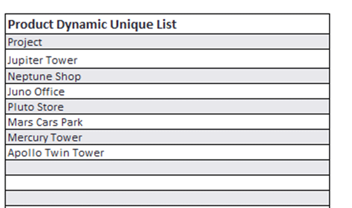
This table contains the name of the projects.

Adding a project here, will automatically add it on the dropdown menu of the Database section/Project field, and it will be selectable for income or expenses allocation.

3.2 Active Staff Table:

This table is vital for the Income, Expenses and Profit allocation.

In this section there is the setup of the percentages used to split the Income, Expenses and Profit between the staff.
This is also a very complex table because the setup will affect from when the Income, Expenses and Profit will be split.

The table has the following columns:

3.2.1 Name

3.2.2 Percentage Cost/Profit

3.2.3 Active

3.2.4 From

3.2.5 To

3.2.6 Active Only

3.2.1 Name:

This column contains the name of staff. Active staff will appear on the 10 Year Tables on the dashboard section. 1. Dashboard

3.2.2 Percentage Cost/Profit:

This column contains the percentages used to calculate the Income, Expenses and Profit for each member of staff.

Please note that the Total Active Staff Sharing should be 100% otherwise it means that costs are over or under split.

3.2.3 Active:

This column makes a member of staff Active or Inactive. Only active members are used for the income/cost calculations.

3.2.4 From:

This column is vital because allows to setup from when a member of staff will take part of the income, expenses and profit sharing.

i.e. in the table above none of the members will get sharing of Income or Costs for transactions that happened before the 01/07/2003.

3.2.5 To:

This column is vital because allows to setup up to when a member of staff will take part of the income, expenses and profit sharing.

i.e. in the table above non of the members will get sharing of Income or Costs for transactions that happened after the 31/12/2013.

The From and To columns can be used to setup the length of a contract for a specific member of staff.

3.2.6 Active Only:

This column is a calculate field and based on the column active, it will recreate a list of active members only.

Active members appear on the Current Band Staff and Income/Costs Allocation Based on Contribution Percentage section on the dashboard.

3.3 Project Table:

This table contains the project for what you want to track costs.

If you need to add a project, please do that on the first empty row below the table. The table will expand automatically and the whole dashboard will update accordingly.

3.4 Other Tables:

In this section there are 3 other tables that are used for calculations and further setup.

The first table called Dates calculation for last year income and expenses is used on the calculations on the Income Summary and Expenses Summary on the Dashboard section. 1. Dashboard

The second and the third table are used to calculate the 10 years period and to change automatically the title of the graph on the dashboard section in the next years

To download the dashboard please click here: Revenues and Costs Tracking Dashboard

Please save the Dashboard on your Computer before using it. Once you have saved the file, unzip it using 7z [http://www.7-zip.org/] and install it.

Following on from the above also note that LockXLS add-in will execute the file with Excel.

I hope you enjoy the spread-sheet.

Paolo

[Copyright © 2012, Paolo Succo]

Timesheet Dashboard

Dear All,

I am very happy to announce I have created a “Timesheets” Dashboard application.

Unlike many versions you can find online are working perfectly, I have developed a new timesheet format. Timesheet 2012 Dashboard has a new and more user friendly way to fill out your timesheet.

Timesheet 2012 Dashboard is a dynamic spread-sheet and needs the macros enabled to be used. If you do not know how to enable the macros, please follow the instruction at the link http://office.microsoft.com/en-us/excel-help/change-macro-security-settings-in-excel-HP010096919.aspx

The dashboard has two dynamic menus which allow you to actively interact with the spread-sheet. The first menu, called Active Control and shown below, gives you the option to select a specif month or all the month. This can be very helpful to avoid to scroll up and down your timesheet or create a PDF of your timesheet.

The second menu, called User Menu and shown below, has 6 buttons:

1. Update: in spite of your timesheet is automatically updated [not in this Demo version, you will get an error saying it cannot find the server instead] as soon as you open it, this button allows to perform a further manual update. Please note that the Demo version is for demostration only. There is a final version which can be used on an intranet to manage the all companies timesheets
2. Email Admin: this button opens your Outlook and allows sending an email to Admin, copying another address as well. You should email Admin if you need help with your timesheet
3. Create PDF: this features allows to create a PDF of the visible area in your timesheet [Selecting All on the Active Control you will PDF the 12 months while selecting only one month you will PDF only the selected month]. The PDF will be automatically saved on your PC with the format FileNameCurrentDate.pdf [Document folder or desktop]
4. Quick timesheet: this button is the most powerful tool on the new timesheet. This control allows to select a range and fill it out with the same number of hours. [further explanation below]
5. Save/Close: Save and close button. Please use this button to save your timesheet and resetup Excel with the normal view
6. Admin: only Admin is allow to use this tool. The spreadsheet automatically recognize who is logged in

The Quick Timesheet tool:

In spite of you still should fill out your timesheet in the “old fashioned” way, and which I strongly recommend to do, I have developed a tool to fill out the timesheet faster.

As already aforementioned, this tool allows you to fill out a range of cells with the same number of hours.

In the example below, the days from 2 to 6 and from 9 to 11 have been selected and the Quick Timesheet Tool will fill them out with 8 hours a day as soon as the OK button is clicked.

You can enter letter as well, i.e. H for Holiday and so forth

IMPORTANT:

On top of your timesheet there are some information about the staff. Title and Location have a scroll-down list [the list is dynamic and updatable if connected to the server].

The project area:

As shown below, you can select a project number through a scroll-down list [the list is dynamic and updatable if connected to the server]. Please note that you can select a maximum 15 different projects per month. Projects without hours or vice versa, are not allowed and you cannot save the timesheet if this happen.

To download the timesheet please click here: Timesheet Dashboard

Please save the Timesheet on your Computer before using it. Once you have saved the file, unzip it using 7z [http://www.7-zip.org/] and install it.

Following on from the above also note that LockXLS add-in will be to execute the file with Excel.

I hope you enjoy the spread-sheet.

Paolo

[Copyright © 2012, Paolo Succo]

Sum of cells depending on cell colour formatting

Hi All,

I recently came out with a problem using the sum function.
Imagine that you have a range of cells and you used a background color to identify certain specific cells and you wish to calculate the sum of only the cells with, for example, the red background in the range.
How can this problem be sorted out? Here the solution:

Function SumColor(DefClr As Range, DefRng As Range)

Dim MyCell As Range
Dim MyCol As Long
Dim SumColCell

'Identify the colored cell
MyCol = DefClr.Interior.ColorIndex

'Sum the colored cells in the range
For Each MyCell In DefRng
If MyCell.Interior.ColorIndex = MyCol Then
SumColCell = WorksheetFunction.SUM(MyCell, SumColCell)
End If
Next MyCell

SumColor = SumColCell

End Function


The VBA formula above as two parameters. With the first one you identify a colored cell in the range that you want to sum, the second is the range that you want to sum.

E.g.

Let's assume that this is what you have on column A:

A1. with red background

A2. with red background

A3. with yellow background

A4. cell with no background

A5. cell with no background

If you want to know the sum of only the red background cells, proceed as follow:

enter in A6 =SumColor(A1,A1:A5)

Enjoy

Comparing Two List

Hey Guys,

having problems in ffinding duplicates between two numerical list?
Here the solution:

Download the two lists comparing spreadsheet

The spreadsheet can be used for text lists as well but it might be possible you need to reformat the texts before comparing them.

Enjoy

2D & 3D Animation With Excel

Hi Guys,

please find enclosed an Excel File showing 2D and 3D animations with Excel.

Download the animation:
2D & 3D Animation with Excel

Enjoy

List Files In A Specif Folder

Hi Guys,

Today I will show you how to select a folder from your computer and list all the files in it.

The Macro will also give you information about the files like:

1 - Name
2 - Size
3 - Date and Time


Sub ListFilesInAFolder()

'######################################################################

'Author Paolo Succo
'Date 12 December 2011

'Macro to list files in a folder

'######################################################################

Dim directory As String
Dim r As Long
Dim f As String
Dim path As String


'Select folder
With Application.FileDialog(msoFileDialogFolderPicker)
.InitialFileName = Application.DefaultFilePath & "\"
.Title = "Please select a location for the file list"
.Show

Range("A:C").Select
Selection.Delete
ActiveSheet.Shapes.Range(Array("Bevel 1")).Select
Selection.ShapeRange.IncrementLeft 150#
Selection.ShapeRange.IncrementTop -0.75

If .SelectedItems.Count = 0 Then
MsgBox "Canceled"
Else
path = .SelectedItems(1)
path = directory


r = 1

'Headers
Cells(r, 1) = "Filename"
Cells(r, 2) = "Size"
Cells(r, 3) = "Date/Time"
Range("a1:c1").Font.Bold = True

'Get file
f = Dir(directory, vbReadOnly + vbHidden + vbSystem)
Do While f <> ""
r = r + 1
Cells(r, 1) = f
Cells(r, 2) = FileLen(directory & f)
Cells(r, 3) = FileDateTime(directory & f)

'get next file
f = Dir()

Loop

End If
End With

Cells.EntireColumn.AutoFit

End Sub

Download an example:

Files_List.xlsm