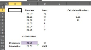
I would like to demonstrate how the well known Excel function VLOOKUP can fail.
Let's assume that we are looking for the value 21.01 in column C and that we want to return the value in column D.

I have created a dropdown list to be sure that the value I am picking up is exactly like the one that is in column C and I have entered my VLOOKUP function to get the letter in column D
=VLOOKUP(C12,$C$3:$D$8,2,0)
As expected, selecting from the dropdown menu 21.01, the VLOOKUP function returns the letter W.
I have then entered in column F three numbers: 7, 0.01 and 14 which the sum is 21.01. In column C I have entered the formula =SUM(F3:F5) [F3:F5 contains the numbers] and in column D there is again my VLOOKUP formula =VLOOKUP(C13,$C$3:$D$8,2,0).
Surprisingly, VLOOKUP returns #N/A.

However, the same example using the number 21.02 doesn't return an error.
How is this possible? Why VLOOKUP is not working? Why the first 21.01 from the dropdown list is different from the 21.01 as a result of a formula?
Here the explanation:
If we consider the decimal part of the two numbers 0.01, we can discover that they are actually different.
The 0.01 from the dropdown list is recognized by Excel as 0.010000000000002 while the one that is calculated is 0.009999999999998. Why is this happening?
This problem occurs because of the precision of your computer, which must represent and manipulate numbers in binary. Microsoft Excel compares the exact binary representation of the numbers, rather than their decimal equivalents, which are displayed on the screen. Therefore, rounding errors can occur in the binary representation of the numbers that are not evident when you compare the decimal values visually.
When storing numbers, a corresponding binary number can represent every number or fractional number. For example, the fraction 1/10 can be represented in a decimal number system as 0.1. However, the same number in binary format becomes the repeating binary decimal 0001100110011100110011 (and so on) and can be infinitely repeated. This number cannot be represented in a finite (limited) amount of space. Therefore, this number is rounded down by approximately -2.8E-17 when it is stored.
All numbers expressed in floating-point format are rational numbers. Irrational numbers such as π or the square root of 2, or non-terminating rational numbers must be approximated. The number of digits of precision also limits the accuracy of the numbers. Excel store 15 significant digits of precision. For example, the number 1234567890123456 cannot be exactly represented if 15 digits of precision are used.
Many combinations of arithmetic operations on floating-point numbers may produce results that appear to be incorrect by very small amounts. For example, the equation
=1*(0.5-0.4-0.1)
may be evaluated to the quantity (-2.78E-17), or -0.0000000000000000278 instead of 0. This is due to the fact that the IEEE 754 standard requires numbers to be stored in binary format. As I described earlier, not all decimal numbers can be converted exactly to binary, as in the case of 0.1. The conversion caused the loss of precision.
Going back to our example, we can see that the 21.01 from the dropdown list is exactly the same of the original list in column C [which is the source for that number], which means that it is affect by the same error, while the one that is calculated is different.
If we convert the decimal part of both numbers as a binary number, we get the following:
Typed 0.01 = 000000101000111101011100001010001111010111000011000000
Calculated 0.01 = 000000101000111101011100001010001111010111000010000000
as you can see, the last 7 digits are different, therefore the numbers are considered by Excel as two different numbers.
To correct the precision error we can change our VLOOKUP formula as follow:
=VLOOKUP(TRUNC(C13,2),$C$3:$D$8,2,0) or =VLOOKUP(ROUND(C13,2),$C$3:$D$8,2,0)
I hope this helps all of you who incurred in this error.
Best,
Paolo